

In this article
The era of Physical AI is no longer a futuristic concept sitting on the pages of science fiction novels. It is happening right now, in warehouses, surgical suites, autonomous vehicles, and agricultural fields across the globe. Physical AI refers to the discipline of deploying intelligent algorithms into machines that operate in and interact with the real physical world. Python has emerged as the lingua franca for this domain, offering a rich ecosystem of tools spanning Robot Operating System (ROS), OpenAI Gym, PyBullet, and Stable-Baselines3. This blog post takes you on a complete technical journey from building and training a robotic agent inside a simulation environment to deploying it on real hardware. Whether you are a robotics engineer, an AI researcher, or a decision-maker evaluating automation investments, this guide will give you a firm grasp of how modern Physical AI pipelines are architected, trained, and shipped.
What is Physical AI?
Physical AI is the convergence of machine learning, control theory, computer vision, and mechanical engineering into systems that can perceive their environment, reason about it, and take physical actions. Unlike traditional software agents that live inside a browser or a cloud server, Physical AI agents operate under real-world constraints such as gravity, sensor noise, latency, and mechanical wear.
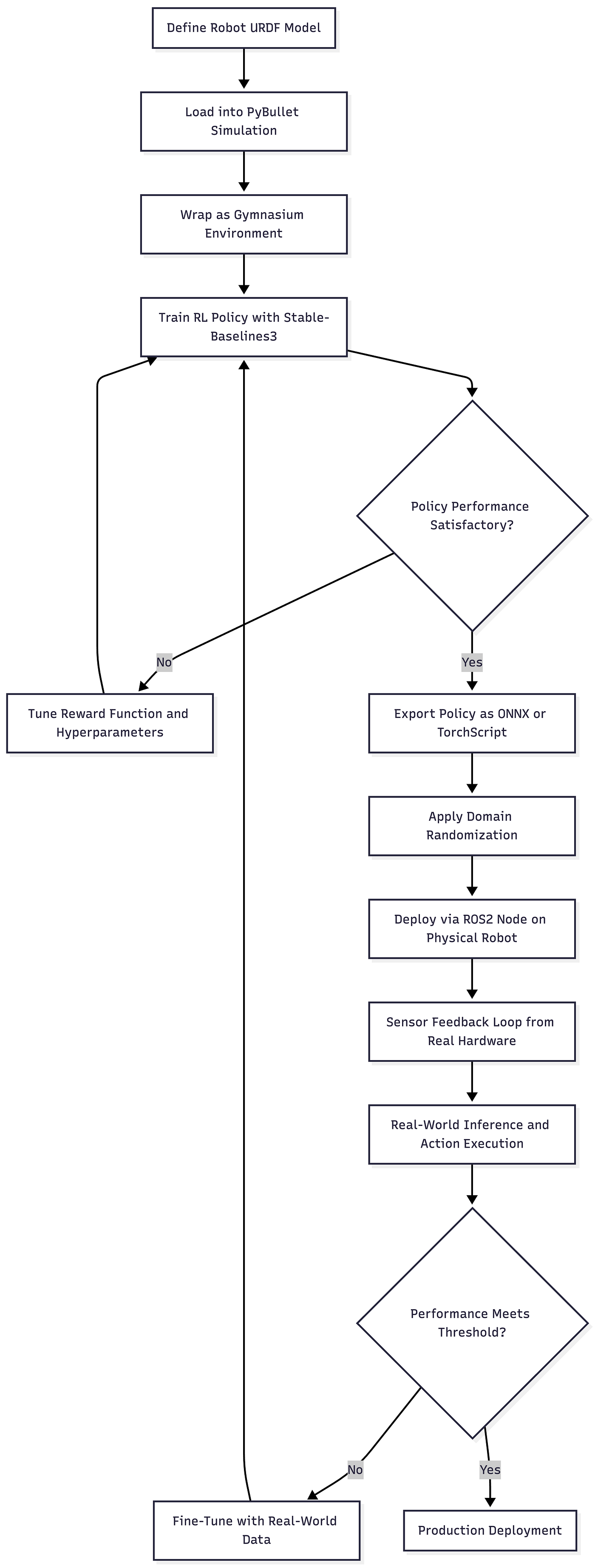
The typical Physical AI development lifecycle follows a sim-to-real pipeline. You train your agent in a simulated world because running thousands of training episodes on a physical robot is slow, expensive, and potentially dangerous. Once the agent achieves reliable performance in simulation, you apply a set of domain adaptation techniques and transfer the policy to the real robot.
Key Tools and Frameworks
Robot Operating System (ROS / ROS2)
ROS is the backbone of modern robotics software. It is a middleware layer that provides standardized communication between sensor nodes, actuator nodes, planning modules, and perception systems. ROS2, the modern successor, offers real-time support, DDS-based communication, and better security primitives. Python bindings via rclpy make it fully accessible to the Python developer community.
OpenAI Gym and Gymnasium
Gymnasium (the maintained fork of OpenAI Gym) provides a standardized environment interface for reinforcement learning. The step(), reset(), and render() API contract allows you to swap between environments without changing your training loop. Robotics-specific Gym environments include MuJoCo, PyBullet-Gym, and Isaac Gym from NVIDIA.
PyBullet
PyBullet is a physics simulation engine that supports rigid body dynamics, soft body simulation, and collision detection. It integrates seamlessly with Gym to create custom robot environments. You can load URDF (Unified Robot Description Format) files to simulate real robot models like the Franka Panda arm or a Boston Dynamics-style quadruped.
Stable-Baselines3 (SB3)
SB3 is the gold standard library for training RL agents in Python. It provides clean, tested implementations of PPO, SAC, TD3, A2C, and DDPG. Combined with Gymnasium and PyBullet, it forms a complete training stack for robotic control policies.
ROS-Gym Bridge
The gym_ros and ros2_gym packages allow your trained Gym-compatible policy to communicate with real robot hardware via ROS topics and services. This bridge is the critical link between the simulation world and physical deployment.
Architecture Overview
The Sim-to-Real Gap
The biggest challenge in Physical AI is the sim-to-real gap. Models trained in simulation encounter unexpected behavior in the real world due to differences in friction coefficients, sensor noise distributions, lighting conditions, and actuator dynamics. The standard mitigation strategies include domain randomization (randomly varying simulation parameters during training), system identification (calibrating simulation parameters to match real hardware), and adaptive control policies that can adjust to environmental shifts at inference time.
Detailed Code Sample with Visualization
The following code builds a complete pipeline for training a robotic arm (simulated as a simplified 2-DOF reacher) using PyBullet and Stable-Baselines3, then shows how to export and wrap the trained policy into a ROS2-compatible structure.
Step 1: Custom PyBullet Gymnasium Environment
# custom_reacher_env.py
# A custom 2-DOF robotic arm environment using PyBullet and Gymnasium

import gymnasium as gym
import numpy as np
import pybullet as p
import pybullet_data
from gymnasium import spaces


class ReacherEnv(gym.Env):
    """
    A simulated 2-DOF reacher robot trained to touch a target position.
    Uses PyBullet physics engine under the hood.
    """

    metadata = {"render_modes": ["human", "rgb_array"], "render_fps": 50}

    def __init__(self, render_mode=None):
        super().__init__()

        self.render_mode = render_mode
        self.dt = 1.0 / 50.0          # physics timestep
        self.goal_threshold = 0.05    # meters: considered "reached" if within 5cm

        # Connect to PyBullet in GUI or DIRECT mode based on render preference
        if render_mode == "human":
            self.physics_client = p.connect(p.GUI)
        else:
            self.physics_client = p.connect(p.DIRECT)

        p.setAdditionalSearchPath(pybullet_data.getDataPath())
        p.setGravity(0, 0, -9.81)

        # Action space: joint velocities for 2 joints, normalized to [-1, 1]
        self.action_space = spaces.Box(
            low=-1.0, high=1.0, shape=(2,), dtype=np.float32
        )

        # Observation: [joint1_angle, joint2_angle, joint1_vel, joint2_vel,
        #               end_effector_x, end_effector_y, goal_x, goal_y]
        self.observation_space = spaces.Box(
            low=-np.inf, high=np.inf, shape=(8,), dtype=np.float32
        )

        self.robot_id = None
        self.goal_pos = None
        self.goal_visual = None

    def _load_robot(self):
        """Load a URDF model. Here we approximate a 2-DOF arm using PyBullet primitives."""
        # Load the plane for visual grounding
        p.loadURDF("plane.urdf")

        # Load a simplified arm model (use kuka arm as proxy for demonstration)
        robot_id = p.loadURDF(
            "kuka_iiwa/model.urdf",
            basePosition=[0, 0, 0],
            useFixedBase=True
        )
        return robot_id

    def _get_end_effector_pos(self):
        """Retrieve the current end-effector (link 6) world position."""
        state = p.getLinkState(self.robot_id, linkIndex=6)
        pos = state[0]  # world position tuple (x, y, z)
        return np.array(pos[:2], dtype=np.float32)  # return x, y only (2D task)

    def _get_obs(self):
        """Construct the observation vector from current robot state."""
        joint_states = p.getJointStates(self.robot_id, jointIndices=[0, 1])
        angles = np.array([s[0] for s in joint_states], dtype=np.float32)
        velocities = np.array([s[1] for s in joint_states], dtype=np.float32)
        ee_pos = self._get_end_effector_pos()
        goal = np.array(self.goal_pos, dtype=np.float32)
        return np.concatenate([angles, velocities, ee_pos, goal])

    def _compute_reward(self):
        """
        Dense reward based on negative distance to goal.
        Sparse bonus reward granted when the agent reaches the goal.
        """
        ee_pos = self._get_end_effector_pos()
        dist = np.linalg.norm(ee_pos - np.array(self.goal_pos))
        reward = -dist  # encourage minimizing distance

        if dist < self.goal_threshold:
            reward += 10.0  # bonus for reaching goal

        return float(reward), dist < self.goal_threshold

    def reset(self, seed=None, options=None):
        super().reset(seed=seed)
        p.resetSimulation()
        p.setGravity(0, 0, -9.81)
        p.setAdditionalSearchPath(pybullet_data.getDataPath())

        self.robot_id = self._load_robot()

        # Randomize goal position (domain randomization lite)
        angle = self.np_random.uniform(0, 2 * np.pi)
        radius = self.np_random.uniform(0.3, 0.6)
        self.goal_pos = [radius * np.cos(angle), radius * np.sin(angle)]

        # Visual marker for the goal
        self.goal_visual = p.createVisualShape(
            p.GEOM_SPHERE, radius=0.04, rgbaColor=[1, 0, 0, 1]
        )

        obs = self._get_obs()
        info = {}
        return obs, info

    def step(self, action):
        """Apply joint velocity actions and advance the simulation by one step."""
        # Scale action from [-1, 1] to actual velocity range
        max_velocity = 0.5  # radians per second
        scaled_action = action * max_velocity

        # Apply velocity control to the first two joints
        for i, vel in enumerate(scaled_action):
            p.setJointMotorControl2(
                bodyIndex=self.robot_id,
                jointIndex=i,
                controlMode=p.VELOCITY_CONTROL,
                targetVelocity=vel,
                force=100
            )

        p.stepSimulation()

        obs = self._get_obs()
        reward, terminated = self._compute_reward()
        truncated = False  # handle via TimeLimit wrapper
        info = {}

        return obs, reward, terminated, truncated, info

    def close(self):
        p.disconnect(self.physics_client)
Step 2: Training the Agent with Stable-Baselines3
# train_agent.py
# Train a PPO agent on the custom reacher environment

import gymnasium as gym
from stable_baselines3 import PPO
from stable_baselines3.common.env_util import make_vec_env
from stable_baselines3.common.callbacks import EvalCallback, CheckpointCallback
from stable_baselines3.common.monitor import Monitor
from gymnasium.wrappers import TimeLimit

from custom_reacher_env import ReacherEnv


def make_env():
    """Factory function: wraps the raw env with Monitor and TimeLimit."""
    env = ReacherEnv(render_mode=None)
    env = TimeLimit(env, max_episode_steps=200)   # 200 steps per episode
    env = Monitor(env)
    return env


# Vectorize 4 parallel environments for faster data collection
vec_env = make_vec_env(make_env, n_envs=4)

# Separate evaluation environment (single instance)
eval_env = make_env()

# Callbacks: save best model and periodic checkpoints
eval_callback = EvalCallback(
    eval_env,
    best_model_save_path="./models/best_model",
    log_path="./logs/eval",
    eval_freq=10_000,         # evaluate every 10k environment steps
    n_eval_episodes=10,
    deterministic=True,
    render=False
)

checkpoint_callback = CheckpointCallback(
    save_freq=50_000,
    save_path="./models/checkpoints/",
    name_prefix="ppo_reacher"
)

# Define PPO agent with tuned hyperparameters for continuous control
model = PPO(
    policy="MlpPolicy",
    env=vec_env,
    learning_rate=3e-4,
    n_steps=2048,          # rollout buffer size per environment
    batch_size=64,
    n_epochs=10,
    gamma=0.99,            # discount factor
    gae_lambda=0.95,       # generalized advantage estimation
    clip_range=0.2,        # PPO clipping parameter
    ent_coef=0.005,        # entropy regularization for exploration
    vf_coef=0.5,
    max_grad_norm=0.5,
    verbose=1,
    tensorboard_log="./logs/tensorboard/"
)

print("Starting training...")
model.learn(
    total_timesteps=500_000,
    callback=[eval_callback, checkpoint_callback],
    progress_bar=True
)

# Save the final trained model
model.save("./models/ppo_reacher_final")
print("Training complete. Model saved.")
Step 3: Exporting the Policy for Deployment
# export_policy.py
# Export the trained SB3 policy as a standalone TorchScript module
# for deployment outside the SB3 framework (e.g., inside a ROS2 node)

import torch
import numpy as np
from stable_baselines3 import PPO


def export_to_torchscript(model_path: str, output_path: str):
    """
    Load a trained SB3 PPO model and export its policy network
    as a TorchScript file that can be loaded anywhere without SB3.
    """
    model = PPO.load(model_path)
    policy = model.policy
    policy.eval()

    # Create a dummy observation matching the environment's obs space (8 dims)
    dummy_obs = torch.zeros(1, 8, dtype=torch.float32)

    # Trace the policy forward pass
    with torch.no_grad():
        traced_policy = torch.jit.trace(
            policy.mlp_extractor,   # the shared feature extractor
            dummy_obs
        )

    traced_policy.save(output_path)
    print(f"TorchScript policy exported to {output_path}")


if __name__ == "__main__":
    export_to_torchscript(
        model_path="./models/ppo_reacher_final",
        output_path="./models/ppo_reacher_policy.pt"
    )
Step 4: ROS2 Inference Node
# ros2_inference_node.py
# A ROS2 Python node that loads the trained policy and controls a real robot.
# Run with: ros2 run your_package ros2_inference_node

import rclpy
from rclpy.node import Node
from sensor_msgs.msg import JointState
from std_msgs.msg import Float64MultiArray

import numpy as np
import torch
from stable_baselines3 import PPO


class ReacherInferenceNode(Node):
    """
    ROS2 node that:
    1. Subscribes to /joint_states to receive real robot sensor data.
    2. Runs inference with the trained PPO policy.
    3. Publishes joint velocity commands to /joint_velocity_controller/commands.
    """

    def __init__(self):
        super().__init__("reacher_inference_node")

        # Load the trained policy model
        self.get_logger().info("Loading trained PPO policy...")
        self.model = PPO.load("./models/ppo_reacher_final")
        self.model.policy.eval()
        self.get_logger().info("Policy loaded successfully.")

        # Goal position (could be received from a goal topic in production)
        self.goal = np.array([0.4, 0.2], dtype=np.float32)

        # Store latest joint state
        self.joint_angles = np.zeros(2, dtype=np.float32)
        self.joint_velocities = np.zeros(2, dtype=np.float32)

        # Subscribe to real robot joint states
        self.joint_state_sub = self.create_subscription(
            JointState,
            "/joint_states",
            self.joint_state_callback,
            10
        )

        # Publisher for joint velocity commands
        self.cmd_pub = self.create_publisher(
            Float64MultiArray,
            "/joint_velocity_controller/commands",
            10
        )

        # Run inference at 50 Hz to match simulation frequency
        self.timer = self.create_timer(0.02, self.inference_step)
        self.get_logger().info("Inference node running at 50 Hz.")

    def joint_state_callback(self, msg: JointState):
        """Parse incoming joint state message from the real robot."""
        if len(msg.position) >= 2:
            self.joint_angles = np.array(msg.position[:2], dtype=np.float32)
            self.joint_velocities = np.array(msg.velocity[:2], dtype=np.float32)

    def _build_observation(self) -> np.ndarray:
        """
        Construct an 8-dimensional observation matching the training environment.
        In a full production system, end-effector position would come from FK or a pose sensor.
        """
        # Simplified FK: approximate ee position from joint angles
        l1, l2 = 0.3, 0.25   # link lengths in meters
        theta1, theta2 = self.joint_angles

        ee_x = l1 * np.cos(theta1) + l2 * np.cos(theta1 + theta2)
        ee_y = l1 * np.sin(theta1) + l2 * np.sin(theta1 + theta2)
        ee_pos = np.array([ee_x, ee_y], dtype=np.float32)

        obs = np.concatenate([
            self.joint_angles,
            self.joint_velocities,
            ee_pos,
            self.goal
        ])
        return obs

    def inference_step(self):
        """Run one inference step: observe, predict, publish."""
        obs = self._build_observation()

        # SB3 expects a batch dimension
        action, _ = self.model.predict(obs, deterministic=True)

        # Clip action to safe velocity range for real hardware
        max_vel = 0.3   # conservative limit for real robot (rad/s)
        safe_action = np.clip(action * max_vel, -max_vel, max_vel)

        # Publish command
        cmd_msg = Float64MultiArray()
        cmd_msg.data = safe_action.tolist()
        self.cmd_pub.publish(cmd_msg)


def main(args=None):
    rclpy.init(args=args)
    node = ReacherInferenceNode()
    try:
        rclpy.spin(node)
    except KeyboardInterrupt:
        node.get_logger().info("Shutting down inference node.")
    finally:
        node.destroy_node()
        rclpy.shutdown()


if __name__ == "__main__":
    main()
Step 5: Visualizing Training Performance
# plot_training_results.py
# Visualize episode reward and distance-to-goal from SB3 monitor logs.

import pandas as pd
import matplotlib.pyplot as plt
import matplotlib.ticker as ticker
import glob
import os


def load_monitor_logs(log_dir: str) -> pd.DataFrame:
    """Load and concatenate all Monitor CSV logs from vectorized envs."""
    files = glob.glob(os.path.join(log_dir, "*.monitor.csv"))
    dfs = []
    for f in files:
        df = pd.read_csv(f, skiprows=1)   # skip the header comment line
        dfs.append(df)
    return pd.concat(dfs).sort_values("t").reset_index(drop=True)


def smooth(values, window=20):
    """Apply a rolling mean for cleaner visualization."""
    return pd.Series(values).rolling(window=window, min_periods=1).mean()


def plot_results(log_dir: str):
    df = load_monitor_logs(log_dir)

    fig, axes = plt.subplots(1, 2, figsize=(14, 5))
    fig.suptitle(
        "PPO Reacher Training Performance",
        fontsize=15, fontweight="bold", y=1.02
    )

    # Plot 1: Episode reward over time
    axes[0].plot(df.index, smooth(df["r"]), color="#2563EB", linewidth=2, label="Smoothed Reward")
    axes[0].fill_between(
        df.index,
        smooth(df["r"]) - df["r"].rolling(20).std().fillna(0),
        smooth(df["r"]) + df["r"].rolling(20).std().fillna(0),
        alpha=0.15, color="#2563EB"
    )
    axes[0].set_title("Episode Reward", fontsize=13)
    axes[0].set_xlabel("Episode")
    axes[0].set_ylabel("Total Reward")
    axes[0].legend()
    axes[0].grid(True, linestyle="--", alpha=0.5)
    axes[0].xaxis.set_major_formatter(ticker.FuncFormatter(lambda x, _: f"{int(x):,}"))

    # Plot 2: Episode length (proxy for task efficiency)
    axes[1].plot(df.index, smooth(df["l"]), color="#16A34A", linewidth=2, label="Smoothed Ep. Length")
    axes[1].set_title("Episode Length (Steps)", fontsize=13)
    axes[1].set_xlabel("Episode")
    axes[1].set_ylabel("Steps to Termination")
    axes[1].legend()
    axes[1].grid(True, linestyle="--", alpha=0.5)
    axes[1].xaxis.set_major_formatter(ticker.FuncFormatter(lambda x, _: f"{int(x):,}"))

    plt.tight_layout()
    plt.savefig("training_results.png", dpi=150, bbox_inches="tight")
    plt.show()
    print("Plot saved as training_results.png")


if __name__ == "__main__":
    plot_results("./logs/")
The chart produced by this script gives you two panels side by side. The left panel shows episode reward increasing and stabilizing as the agent learns to reach the target reliably. The right panel shows episode length decreasing over time, which means the agent is finding the goal faster as training progresses. Both together confirm that the policy is converging correctly before you commit to real-world deployment.
Pros of Physical AI with Python, ROS, and Gym
- Rapid Prototyping at Low Cost. Simulation environments like PyBullet and MuJoCo allow teams to run millions of training episodes at near-zero hardware cost, dramatically reducing the development cycle before any physical component is touched.
- Modular, Reusable Architecture. ROS2 nodes are independently deployable and replaceable. You can swap a camera driver, a planning module, or an inference node without rewiring the entire system.
- Massive Open-Source Ecosystem. The Python robotics ecosystem benefits from thousands of community-maintained packages, pre-trained URDF models, and reference implementations on GitHub that accelerate development significantly.
- Safety-First Training Paradigm. Training in simulation first protects expensive hardware from damage during the exploration phase of reinforcement learning, where agents frequently take suboptimal or random actions.
- Standardized RL Interface via Gymnasium. The Gym API ensures that any trained agent can be tested across dozens of environments with zero code changes, making it easier to benchmark and compare policies.
- Scalable Infrastructure. Vectorized training across multiple CPU or GPU-backed simulation instances scales linearly with compute resources, enabling faster experiments and better final policies.
- Cross-Platform Portability. Policies exported as ONNX or TorchScript can be deployed on edge hardware, including ARM-based embedded systems, NVIDIA Jetson boards, and custom FPGAs, without dependency on full Python environments.
- Strong Domain Randomization Support. Python’s flexibility makes it easy to inject randomness into simulation parameters such as friction, mass, lighting, and sensor noise, which directly improves real-world robustness.
Industries Using Physical AI with ROS and Python
Healthcare and Surgical Robotics
Companies like Intuitive Surgical and Medtronic are integrating AI-driven motion planning into robotic surgery platforms. Python-based simulation pipelines allow surgeons and engineers to pre-validate robotic trajectories in virtual anatomical models before any procedure. Reinforcement learning policies trained in simulation are increasingly being evaluated for tasks like tissue retraction, suture assistance, and instrument navigation in minimally invasive surgeries.
Automotive and Autonomous Vehicles
Self-driving companies, including Waymo, Cruise, and Mobileye, use simulation-first pipelines extensively. While their stacks often rely on proprietary simulators, the principles are identical: train perception and planning models in simulation, validate in structured testing environments, then deploy on physical vehicles. Python, ROS2, and custom Gym environments are standard tools in their data-to-deployment pipelines.
Logistics and Warehousing
Amazon Robotics, Ocado, and Mujin use robotic pick-and-place systems that are trained using reinforcement learning in simulated warehouse environments. Tasks such as grasping irregularly shaped items, navigating dynamic shelving environments, and coordinating multi-robot fleets benefit enormously from sim-to-real RL pipelines built in Python.
Agriculture and Precision Farming
Startups like Carbon Robotics and FarmWise deploy intelligent field robots that identify and eliminate weeds using computer vision and precise actuator control. These robots are trained in simulated field environments and deployed on real agricultural machinery. ROS2 handles the real-time sensor fusion between LIDAR, GPS, and vision systems while Python models drive decision-making.
Manufacturing and Quality Control
ABB, FANUC, and Universal Robots integrate adaptive control policies trained with RL into their industrial arms. Tasks like adaptive welding path planning, assembly force control, and visual defect detection benefit from policies trained in simulation and deployed via ROS2 interfaces on real factory floors. Python-based vision pipelines using OpenCV and torchvision operate in the same ROS2 node graph as the control systems.
Defense and Search and Rescue
Autonomous UAVs and ground robots used in disaster response scenarios rely on sim-to-real training to learn navigation in rubble, unstable terrain, and GPS-denied environments. ROS2 provides the communication layer between onboard sensors, the planning stack, and the human operator interface, while Python-based RL policies govern local navigation decisions.
How PySquad Can Assist in This
Physical AI is a demanding discipline that requires deep expertise across reinforcement learning, robotics middleware, systems engineering, and hardware integration. PySquad brings all of these capabilities together under one roof, giving organizations a reliable partner to navigate the full journey from concept to deployment.
- PySquad has built custom ROS2 node architectures for clients across logistics, manufacturing, and healthcare sectors, ensuring that simulation-trained policies translate cleanly to real hardware control loops with minimal performance degradation.
- PySquad specializes in Gymnasium environment design from scratch. Whether you need a custom URDF robot model, a domain-randomized training curriculum, or a multi-agent coordination environment, PySquad engineers design environments tailored to your exact robot hardware and task requirements.
- PySquad has hands-on experience with Stable-Baselines3, RLlib, and CleanRL for training continuous control policies. PySquad knows which algorithm to use for which task type and how to tune hyperparameters efficiently to reduce your compute budget without sacrificing policy quality.
- PySquad handles the full sim-to-real pipeline. From PyBullet simulation setup and URDF calibration to TorchScript export and edge deployment on Jetson-class hardware, PySquad manages every step of the transition.
- PySquad builds robust domain randomization strategies that bridge the sim-to-real gap proactively. Rather than discovering deployment failures after the fact, PySquad stress-tests policies against a wide distribution of environmental parameters before any physical rollout begins.
- PySquad integrates Physical AI pipelines with enterprise data systems. Whether your team needs a ROS2 fleet management dashboard, a real-time telemetry pipeline, or a cloud-based training orchestration system, PySquad connects the robotics layer with your broader technology infrastructure.
- PySquad’s safety-first engineering culture means that every deployment checklist includes hardware-in-the-loop testing, velocity limit validation, emergency stop protocols, and fail-safe recovery behaviors before any robot is authorized to operate autonomously near humans.
- PySquad offers end-to-end project delivery from requirements scoping through prototyping, iteration, deployment, and ongoing support. PySquad does not hand you a trained model and walk away. PySquad stays engaged through integration, monitoring, and the inevitable edge cases that arise in production environments.
- PySquad’s team of Python specialists and ML engineers means you get cross-disciplinary expertise in a single engagement. PySquad eliminates the coordination overhead of working with multiple specialist vendors.
- Organizations that partner with PySquad gain not only a delivered solution but also internal knowledge transfer, documented codebases, and trained internal teams. PySquad believes that empowering your engineers is as important as shipping the software.
References
- ROS2 Official Documentation and Tutorials
The primary reference for all ROS2 concepts, node architecture, DDS communication, and Python bindings viarclpy. - Farama Foundation Gymnasium Documentation
Official documentation for the Gymnasium RL environment interface, environment wrappers, and the full catalog of built-in and community environments. - Stable-Baselines3 Documentation and GitHub Repository
Comprehensive documentation for SB3 algorithms, custom policy networks, vectorized environments, callbacks, and export utilities. - PyBullet Physics Engine Documentation
Reference guide for PyBullet simulation, URDF loading, joint control modes, and collision detection APIs. - OpenAI Spinning Up: Introduction to RL
A foundational resource for understanding the RL algorithms (PPO, SAC, TD3) used in robotic control policy training. - NVIDIA Isaac Gym: Technical Report
Whitepaper covering GPU-accelerated robot learning environments and their applications in sim-to-real transfer at scale.
Conclusion
Physical AI represents one of the most consequential intersections of software and the physical world that our industry has ever attempted. The combination of Python’s accessible syntax and rich ecosystem, ROS2’s battle-tested robotics middleware, and Gymnasium’s standardized RL interface gives practitioners a genuinely capable toolkit for building intelligent machines that operate outside of server racks and into the real world.
The pipeline we walked through in this post covers the full arc of a real Physical AI project: designing a custom simulation environment, training a reinforcement learning policy with Stable-Baselines3, exporting that policy for deployment, wiring it into a ROS2 node that communicates with real hardware, and visualizing training progress to validate convergence. Each of these steps has its own depth, and each one matters for whether your agent succeeds or fails when it finally meets the unpredictable real world.